The Fast Fourier Transform over finite fields

The Fast Fourier Transform (FFT) developed by Cooley and Tukey in 1965 has its origins in the work of Gauss. The FFT, its variants and extensions to finite fields, are a fundamental algorithmic tool and a beautiful example of interplay between algebra and combinatorics. There are many great resources on FFT, see ingopedia’s curated list.

Given a field $F$, a polynomial of degree at most $d-1$ is defined as $P(X)=a_0+a_1 X+ \dots + a_{d-1} X^{d-1}$, where each $a_i \in F$. $P(X)$ can be viewed as a vector $\vec{a}=\langle a_0,\dots,a_{d-1} \rangle$ of $d$ elements in $F$.

Polynomials can also be evaluated. Given $d$ unique points $x_1,\dots,x_d$ in $F$, we can represent $P(X)$ as the vector $\vec{y}=\langle y_1,\dots,y_d \rangle$, where $y_i=P(x_i)$ is the evaluation of $P(X)$ on $x_i$.

In a previous post we showed the isomorphism $\vec{a} \leftrightarrow \vec{y}$ between degree at most $d-1$ polynomials and their evaluations at $d$ unique points. Here we focus on the computational cost of this mapping: the number of field operations.

Given $\vec{a}$ for a polynomial of degree at most $d-1$, one can compute each $y_i=P(x_i)$ using Horner’s method via $O(d)$ field operations (observing that $P(X)=a_0+x(a_1+(x(a_2 + \dots + )))$ ). For a total of $O(d^2)$ operations to compute $\vec{y}$. Can we compute the evaluation $\vec{a} \to \vec{y}$ in better than quadratic?

Similarly, for $d$ unique points $\vec{x}$, it is possible to compute the $i$-th Lagrange base polynomial $L_i(X)$ which equals 1 on $x_i$ and 0 for all $x_j, j \neq i$ using $O(d)$ operations as $L_i(X)= \prod_{j \neq i} (X-x_j)/ \prod_{j \neq i} (x_i-x_j)$. So given evaluations $\vec{y}$, computing $P(X)= \sum_{i=1}^d y_i L_i(X)$ can be done in $O(d^2)$ operations. Can we compute the interpolation $\vec{y} \to \vec{a}$ in better than quadratic?

The Fast Fourier Transform allows interpolating and evaluating a polynomial on special points, roots of unity, with $O( d \log d)$ operations.

FFT Theorem:

• Given $d=2^D$ and a field $F$ of characteristic $p=qd+1$, let $\omega$ be a primitive $d$-th root of unity. There exists as algorithm that in $O(d \log d )$ operations:
• Computes $P(\omega^0),\dots,P(\omega^{d-1})$ given the coefficients of a degree at most $d-1$ polynomial $P(X)$.
• Computes the coefficients of the degree at most $d-1$ polynomial $P(X)$ given $d$ evaluations $P(\omega^0),\dots,P(\omega^{d-1})$.

This result uses two powerful ingredients: divide-and-conquer, and roots of unity. We start with the first direction: computing the evaluations given the coefficients.

The first ingredient: decompose a polynomial into its odd and even coefficients each with half the degree

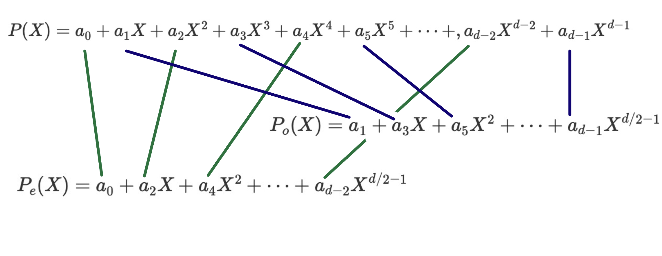
Assume that $P(X)$ has degree at most $d-1$ and that $d=2^D$ is a power of two. A classic divide-and-conquer algorithm design principle when applied to polynomials is to “split” a degree at most $d-1$ polynomial into two degree at most $d/2-1$ polynomials by dividing the polynomial to its even and odd coefficients:

Where $P_e(X),P_o(X)$ are polynomials induced by the even and odd coefficients of $P(X)$ as follows:

Here is a pictorial representation of the odd and even indexes:

Why is this such a powerful divide-and-conquer decomposition?

• Given $d$ evaluations $P_e(a_1^2),\dots,P_e(a_{d}^2)$ and $d$ evaluations $P_o(a_1^2),\dots,P_o(a_{d}^2)$, one can compute the desired $d$ evaluations $P(a_1),\dots,P(a_d)$ in $2d$ operations, simply because $P(a_i)=P_e(a_i^2) + a_i P_o(a_i^2)$ via $(\ref{\star})$.
• The degree of $P_e(X)$ and $P_o(X)$ is at most $d/2-1$. So if we manage to repeat this recursion we can get $O(\log d)$ depth!
• However, to continue recursively there seems to be a challenge:
  • $P_e(X)$ and $P_o(X)$ are of degree less than $d/2$, so from the recursion, we are given only $d/2$ (not $d$) evaluations $P_e(b_1),\dots,P_e(b_{d/2})$ and similarly $d/2$ (not $d$) evaluations for $P_o(X)$.
  • However, to compute all $d$ evaluations of $P(X)$ via $(\ref{\star})$ we need the $d$ evaluations $P_e(a_0^2),\dots,P_e(a_{d}^2)$ and similarly the $d$ evaluations of squares for $P_o(X)$.
• How can we generate $d$ evaluations of squares from just $d/2$ evaluations using $O(d)$ operations?

The second ingredient: use roots of unity

For $g \in F$, if $g^d=1$ then we call $g$ a $d$-th root of unity. Moreover, if $g^1,\dots,g^d$ generates $d$ distinct elements then we call $g$ a primitive $d$-th root of unity.

Suppose $g$ is such a primitive $d$-th root of unity. So $g,g^2,\dots, g^{d-1}, g^d=1$ forms a cyclic group of order $d$ with $d=2^D$.

Now, if we start squaring these roots of unity, we can see a pretty cool pattern. Starting at the first elements, we get:

Since we got to the value $1$ at the $d/2$-th power, elements now start repeating!

So we can solve the challenge above:

• Evaluate $P_e(X)$ and $P_o(X)$ at the $d/2$ points $g^2,g^4, \dots, g^{d}=1$ that form the cyclic group of order $d/2$ of the $d/2$-th roots of unity. Repeating this sequence twice gives us $d$ evaluations at the squares of the cyclic group of order $d$. Each member of $d/2$ appears twice in the squares of $d$:

The $d/2$ evaluations of the $d/2$-th roots, repeated twice, give all the $d$ evaluations of squares of the $d$-th roots. This was the missing piece to complete the divide-and-conquer!

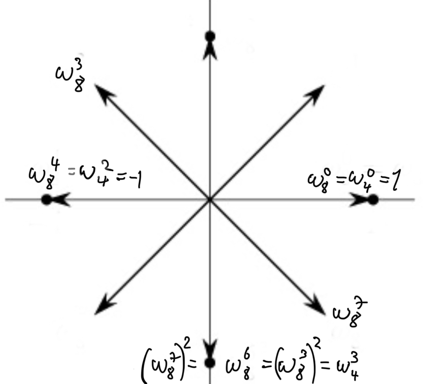
As a visual example, fix $d=8$, every square of a power of $\omega_8$, say $(\omega_8^i)^2$ equals a power of $\omega_4$ (in particular $\omega_4^{i \bmod 4}$). For a specific example consider the squares of $\omega_8^3$ and $\omega_8^7$. Observe that $(\omega_8^3)^2 = \omega_8^6 = \omega_4^3$ and similarly $(\omega_8^7)^2 = \omega_8^{14} = \omega_8^{6} = \omega_4^3$:

Finding a primitive root of unity

If $F$ is a prime Field of characteristic $p=dq+1$ then we are guaranteed that for any $x$, $g=x^q$ is a $d$-th root of unity because $g^d = x^{qd}=x^{p-1}=1$ (using Fermat’s little theorem). It is easy to check that the $d$-th roots of unity form a multiplicative group, and hence a cyclic group.

Choosing $x$ uniformly at random from $F\setminus {0}$ we get that $x^q$ is a uniformly random $d$-th roots of unity.

To see why this is true, denote $f(x)=x^q$ and see that $|x \text{ s.t. } f(x)=y|=q$ for all $y$. Indeed $f(x)$ maps a set of size $dq$ to a set of size at most $d$ (since $f(x)^d=1$ is a root of $x^d -1$ which can have at most $d$ roots). Finally, for any $y$ there can be at most $q$ values such that $x^q=y$. So $f(x)$ must map exactly $q$ elements to each of the $d$ options. Here we used twice the fundamental fact that nontrivial polynomials cannot have more roots than their degree.

Since $d=2^D$, the cyclic group of order $d$ has $d/2$ primitive roots (all the odd powers are generators). Moreover, if $g=x^q$ is not a primitive root, then it’s an even power, so $g^{d/2} = 1$.

That implies a simple Las Vegas algorithm: Randomly choose a nonzero $x \in F$, set $g=x^q$, and if $g^{d/2} \neq 1$ then output $g$, otherwise repeat. Since the probability of success is $1/2$, the expected number of rounds is 2.

Computational cost of the FFT

Each time the degree is cut by half, the depth is $\log_2 d = D$. In each layer, there are $O(d)$ operations: at layer $i$ there are $2^i$ polynomials of degree $2^{d-i}$, each pair of polynomials requires $2^{d-i+2}$ operations to compute the degree $2^{d-i+1}$ polynomial. For a total of $2^{i-1} \times 2^{d-i+2}= 2d$ operations.

So overall $2 d \log_2 d$ field operations.

Interpolation: inverse FFT

Given $d$ evaluations $P(\omega^1),\dots,P(\omega^d)$ can we interpolate and compute the coefficients $\vec{a}$ of $P(X)$ in $O(d \log d)$ operations? Yes, using the same two ingredients!

Let’s look again at

If we had $d/2$ evaluations, $P_e(\omega^2),P_e(\omega^4),\dots,P_e(\omega^d)$ and $d/2$ evaluations, $P_o(\omega^2),P_o(\omega^4),\dots,P_o(\omega^d)$ then we could recursively obtain the coefficients $\vec{b},\vec{c}$ of $P_e(X)$ and $P_o(X)$ respectively.

Now via $(\ref{\star})$ get that $a_{2i}=b_i$ and $a_{2i-1}=c_i$ directly.

So the only challenge is to compute $\vec{e}=P_e(\omega^2),P_e(\omega^4),\dots,P_e(\omega^d)$ and $\vec{o}=P_o(\omega^2),P_o(\omega^4),\dots,P_o(\omega^d)$ from $\vec{y}=P(\omega^1),\dots,P(\omega^d)$.

As expected we will use the properties of roots of unity.

For any $1 \le j \le d/2$ to compute $o_j$ and $e_j$ we start with two equations by evaluating $(\ref{\star})$ at $\omega^j$ and $\omega^{d/2+j}$:

and

Where in the second equation we use $\omega^{d+x}=\omega^x$ and $\omega^{d/2+x}= -\omega^x$. The latter follows from $\omega^{d/2}=-1$ which can be derived from $(\omega^{d/2})^2 -1 =0 = (\omega^{d/2}-1)(\omega^{d/2}+1)$. Now note that $\omega^{d/2} -1 \neq 0$ because $\omega$ is a primitive $d$-th root of unity, so it must be that $\omega^{d/2} + 1 = 0$.

Using the notation $y,e,o$ we get:

and

Adding $(9)$ to $(10)$ and then dividing by 2 we get:

While subtracting $(10)$ from $(9)$ and then dividing by $2\omega^j$ we get:

So we can compute $e_j,o_j$ using a constant number of field operations on $y_j,y_{d/2+j}, \omega^j$, hence compute all of them in $O(d)$ operations.

Again we have $\log_2 d$ layers of recursion and each layer requires $O(d)$ operations for a total of $O(d \log d)$ operations.

Inverse FFT via Inversion

The FFT is a linear transformation of the Vandermonde matrix where $V_{i,j}=\omega^{ij}$. The inverse matrix is $U_{i,j}= \omega^{-ij}/d$. This can be seen as the $i,j$ value of the product $VU$ is $(VU)_{i,j} = \frac{1}{d} \sum_k \omega^{k(i-j)}$ which equals 1 for $i=j$ and 0 otherwise (because $(\omega -1 )(1+\omega+\dots+\omega^{d-1}) = \omega^d -1 = 0$). Hence running the regular FFT with $\omega^{-1}$ and dividing by $d$ is the same as multiplying by the inverse $U$. This obtains inverse FFT as well.

Do we need fields of characteristic $q 2^D+1$?

The requirement to have a field of characteristic $q 2^D+1$ is limiting. What if we are using a field that does not have a large power of two as a root of unity, but we still want to work with large, degree at most $d-1$ polynomials? Recent work of Ben-Sasson, Carmon, Kopparty, and Levit shows how to do FFT for any field in $O(d \log d)$ operations!

Acknowledgments

Many thanks to Gilad Stern, Valeria Nikolaenko, and Dan Boneh for insightful discussions and comments.

Your comments and thoughts on x.