What is a Merkle Tree?

In this post, we will demystify Merkle trees using three examples of problems they solve:

1. Maintaining integrity of files stored on Dropbox.com, or file outsourcing,
2. Proving a transaction between Alice and Bob occurred, or set membership,
3. Transmitting files over unreliable channels, or anti-entropy.

$$ \def\mht{\mathsf{MHT}} \def\mrh{h_{\mathsf{root}}} \def\vect#1{\boldsymbol{\vec{#1}}} $$

By the end of the post, you’ll be able to understand key concepts that, at this point, might intimidate you:

1. A Merkle tree is¹ a collision-resistant hash function, denoted by $\mht$, that takes $n$ inputs $(x_1, \dots, x_n)$ and outputs a Merkle root hash $h = \mht(x_1, \dots, x_n)$,
2. A verifier who only has the root hash $h$ can be given an $x_i$ and an associated Merkle proof which convinces them that $x_i$ was the $i$th input used to compute $h$.
   • In other words, convinces them that there exist other $x_j$’s such that $h=\mht(x_1, \dots, x_{i-1}, x_i,x_{i+1},\dots,x_n)$.
   • This ability to verify that an $x_i$ is the element at the $i$th position against the root hash $h$ (i.e., without having to store all $n$ inputs) is the fundamental power of Merkle trees which we explore in this post.
3. If a Merkle proof says that $x_i$ was the $i$th input used to computed $h$, no attacker can come up with another Merkle proof that says a different $x_i’\ne x_i$ was the $i$th input.
   • More formally, an attacker cannot come up with a Merkle root $h$ and two values $x_i\ne x_i’$ with proofs $\pi_i$ and $\pi_i’$ that both verify for position $i$ w.r.t. $h$.

Prerequisites

Merkle trees are built using an underlying cryptographic hash functions, which we assume you understand. If not, just read our post on hash functions!

Definition: A hash function $H$ is collision resistant if it is computationally-intractable² for an adversary to find two different inputs $x$ and $x’$ with the same hash (i.e., with $H(x) = H(x’)$).

Notation:

• We often use $[k] = \{1,2,\dots, k\}$ and $[i,j] = \{i, i+1,\dots,j-1,j\}$.
• Although a hash function $H(x)$ is formalized as taking a single input $x$, we often invoke it with two inputs as $H(x,y)$. Just think of this as $H(z)$, where $z=(x\ |\ y)$ and $|$ is a special delimiter character.

This is a Merkle tree!

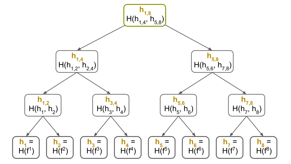
Suppose you have $n=8$ files, denoted by $(f_1, f_2, \dots, f_8)$, you have a collision-resistant hash function $H$ and you want to have some fun.

You start by hashing each file as $h_i = H(f_i)$:

You could have a bit more fun by continuing to hash every two adjacent hashes:

You could even go crazy and continue on these newly obtained hashes:

In the end, you only live once, so you’d better hash these last two hashes as $h_{1,8} = H(h_{1,4}, h_{4,8})$:

Congratulations! What you have done is computed a Merkle tree on $n=8$ leaves, as depicted in the picture above.

Note that every node in the tree stores a hash:

• The $i$th leaf of the tree stores the hash $h_i$ of the file $f_i$.
• Each internal node of the tree stores the hash of its two children.
• The $h_{1,8}$ hash stored in the root node is called the Merkle root hash.

You could easily generalize and compute a Merkle tree over any number $n$ of files.

It is useful to think of computing the Merkle tree as computing a collision-resistant hash function, denoted by $\mht$, which takes $n$ inputs (e.g., the $n$ files) and outputs the Merkle root hash. For example, we will often use the following notation:

Importantly, note that computing $\mht$ (i.e., computing the Merkle tree), involves many computations of its underlying collision-resistant hash function $H$.

At the risk of overwhelming you with notation, it is useful to observe that $h_{1,8}$ has a “recursive” structure:

\begin{align*} h_{1,8} = MHT(f_1, \dots, f_8) = H(\\
& & H(\\
& & & & H(H(f_1), H(f_2)),\\
& & & & H(H(f_3), H(f_4)),\\
& & ),\\
& & H(\\
& & & & H(H(f_5), H(f_6)),\\
& & & & H(H(f_7), H(f_8)),\\
& & )\\
) \end{align*}

Really this is just a (verbose) mathematical representation of the Merkle tree that we visually depicted above!

We often refer to a file $f_i$ as “being in the Merkle tree” to indicate it was one of the $n$ input files used to compute the tree.

This is a Merkle proof!

Alright, you’ve computed your Merkle tree over your 8 files.

Next, you upload your files and Merkle tree on Dropbox.com and delete everything from your computer except the Merkle root $h_{1,8}$. Your goal is to later download any one of your files from Dropbox and make sure Dropbox did not accidentally corrupt it.

This is the file integrity problem and Merkle trees will help you solve it.

The key idea is that, after you download $f_i$, you ask for a small part of the Merkle tree called a Merkle proof. This proof enables you to verify that the downloaded $f_i$ was not accidentally or maliciously modified.

But how do you verify?

Well, observe that the Merkle proof for $f_i$ is exactly the subset of hashes in the Merkle tree that, together with $f_i$, allow you to recompute the root hash of the Merkle tree and check it matches the real hash $h_{1,8}$, without knowing any of the other hashed files.

So, to verify the proof, you simply “fill in the blanks” in the picture above by computing the missing hashes depicted with dotted boxes, in this order: \begin{align*} h_3’ &= H(f_3)\\
h_{3,4}’ &= H(h_3’, h_4)\\
h_{1,4}’ &= H(h_{1,2}, h_{3,4}’)\\
h_{1,8}’ &= H(h_{1,4}’, h_{5,8}) \end{align*}

Lastly, you check that the Merkle root $h_{1,8}’$ you computed above is equal to the Merkle root $h_{1,8}$ you kept locally! If that’s the case, then you can be sure you downloaded the correct $f_i$ (and we prove this later).

But why does this check suffice as a proof that $f_i$ was downloaded correctly? Here’s some intuition. Since the Merkle proof verified, this means you were able to recompute the root hash $h_{1,8}$ by using $f_i$ as the $i$th input and the Merkle proof as the remaining inputs. If the proof verification had yielded the same hash $h_{1,8}$ but with a different file $f_i’ \ne f_i$ as the $i$th input, then this would yield a collision in the underlying hash function $H$ used to build the tree. This last observation is not trivial to see but we will help you see it later, when we argue security formally.

Why use large Merkle proofs anyway?

Forget the Merkle tree! Since you only have eight files, you could check integrity by storing their hashes $h_i=H(f_i)$ rather than their Merkle root $h_{1,8} = \mht(f_1, \dots, f_8)$. After all, the $h_i$ hashes are much smaller than the files themselves.

Then, when you download $f_i$, you hash it as $y_i = H(f_i)$ and check that $h_i = y_i$. Since $H$ is collision-resistant, you can be certain that $f_i$ was not modified. (Indeed, we already discussed how hash functions can be used for download file integrity in our previous post.)

One advantage of this approach is you no longer need to download Merkle proofs.

Unfortunately, the problem with this approach is you have to store $n$ hashes when you outsource $n$ files. While this is fine when $n=8$, it is no so great when $n=1,000,000,000$!

“But that’s crazy! Who has one billion files?” you might protest.

Well, just take a look at the Certificate Transparency (CT) project, which builds a Merkle tree over the set of all digital certificates of HTTPS websites. These Merkle trees easily have hundreds of millions of leaves and are designed to scale to billions.

Moral of the story: To avoid the need for the verifier to store a hash for each one of the $n$ outsourced file, we use Merkle trees. This way, you only need to store a Merkle root hash (rather than $n$ hashes) and receive an $O(\log{n})$-sized Merkle proof with each downloaded file.

If you are still concerned about large Merkle proof size, you should look at more algebraic vector commitments (VCs), such as recent ones based on polynomial commitments or on RSA assumptions. However, be aware that VCs come with their own performance bottlenecks and other caveats.

What else is a Merkle tree useful for?

Now that we know how a Merkle tree is computed and how Merkle proofs work, let’s dig into a few more use-cases.

Efficiently proving Bitcoin transactions were validated

Recall that a Bitcoin block is just a set of transactions that were validated by a miner.

Problem: Sometimes it is useful for Alice, who is running Bitcoin on her mobile phone, to verify that she received a payment transaction from Bob.

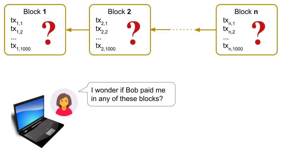
Inefficient, consensus-based solution: Alice could simply download every newly mined Bitcoin block on her phone and inspect the block for a transaction from Bob that pays her. But this requires Alice to download a lot of data (1 MiB / block), which can be either slow or expensive, since mobile data costs money. (The unstated assumption here is that Alice relies on Bitcoin’s proof-of-work consensus protocol to decide whether a block is valid. These consensus-related details are covered in other posts³$^,$⁴ on this blog.)

Insecure, polling-based solution: Note that Alice cannot just simply ask nodes on the Bitcoin network, “Hey, was I paid by Bob?” since nodes can lie and say “Yes, you were” showing her a transaction from Bob that is actually not yet incorporated into a block.

Efficient, Merkle-based solution: If Alice was indeed paid by Bob, then Bitcoin can prove this to her via a Merkle proof. Specifically, Alice will ask a Bitcoin node if she was paid by Bob in the latest block, but instead of simply trusting the “Yes, you were paid and here’s the transaction” answer, she will ask the node to prove membership of the transaction in the block via a Merkle proof.

Importantly, Alice never has to download the full block: she only needs to download a small part of the block called the block header, which contains the root of a Merkle tree built over all transactions in that block⁵. This way, Alice can verify the Merkle proof leading to Bob’s transaction in this tree, which will assure her that Bob’s transaction is in the block without having to download the other transactions.

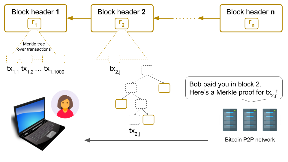
This Merkle-based solution still requires Alice to rely on Bitcoin’s proof-of-work consensus to validate block headers. However, since headers are 80 bytes, this is much more efficient than downloading full (1 MiB) blocks. Furthermore, some of you might note that, because of Bitcoin’s chronologically-ordered Merkle tree, a node can still lie and say “No, you weren’t paid by Bob” and Alice would have no way to tell the truth efficiently without actually downloading every new block and inspecting it. One way this problem could be solved is by re-ordering Bitcoin’s Merkle tree, either by the payer or by the payee’s Bitcoin address. We leave the details of this to another post.

Moral of the story: The beauty of Merkle trees is that a prover, who has a large set of data (e.g., thousands of transactions) can convince a verifier, who has access to the set’s Merkle root hash, that a piece of data (e.g., a single transaction) is in this large set by giving the verifier a Merkle proof.

Downloading files over corrupted channels, or anti-entropy via Merkle trees

In our previous example, we showed how you could outsource your files to Dropbox and detect malicious or accidental modifications of any of your files.

Suppose the modifications were accidental due to an unreliable connection to Dropbox. It would be nice if you could not just detect these modifications but actually recover from them and eventually download the original, unmodified file.

The naive solution would be to simply restart the file download whenever you detect a modification via the Merkle-based technique we discussed before. However, this could be painfully slow. In fact, if the connection is sufficiently unreliable and if the file is sufficiently large, this might never terminate.

A better solution is to split the file into blocks and use the Merkle tree to detect modifications at the block level (i.e., at a finer granularity) rather than at the file level. This way, you only need to restart the download for incorrectly downloaded blocks, which helps you make steady progress.

To keep things simple, we will focus on a simpler scenario where just one file is outsourced to Dropbox rather than $n$ files. We will discuss later how this can be generalized to $n$ files.

Inefficient: Recovering corrupted file blocks with one Merkle proof per block

As we said above, we will split the file $f$ into, say, $b=8$ blocks:

Then, we will build a Merkle tree over these 8 blocks:

As before, you send $f$ and the Merkle tree to Dropbox, and you store $h_{1,8}$ locally.

Next, to download $f$ reliably, you will now download each block of $f$ with its Merkle proof, which you verify as discussed in the beginning of the post. And if a block’s proof does not verify, you ask for that block and its proof again until it does. Ultimately, the unreliable channel will become reliable and the proof will verify.

This approach is better than the previous one because, when the channel is unreliable, you do not need to restart the download of $f$ from scratch. Instead, you only restart the download for the specific block of $f$ that failed downloading.

Note that there’s an interesting choice of block size to be made, as a function of the unreliability of the channel. However, this is beyond the purpose of this post. Also note that there are other ways to deal with unreliable channels, such as error-correcting codes, which again are beyond the purpose of this post.

Unfortunately, in this first solution, you are re-downloading the full Merkle tree, in addition to the blocks themselves. This is because Dropbox sends a Merkle proof for every block⁶, even if that block is correct.

We will fix this next.

Recovering corrupted file blocks with one Merkle proof per corrupted block

A better solution is to observe that you can first optimistically download all $b=8$ blocks, and rebuild the Merkle tree over them. If you get the same root hash $h_{1,8}$, you have downloaded the file $f$ correctly and you are done!

Otherwise, let’s go through an example to see how you would identify the corrupted blocks. Assume, for simplicity, that only block $5$ (denoted by $f^5$) is corrupted. Then, the Merkle tree you re-compute during the download would differ only slightly from the one you originally computed above.

Specifically, you would re-compute the tree below, with the difference highlighted in red:

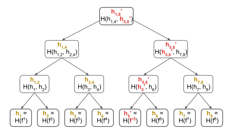
If all blocks were correct, you expect the root hash of the Merkle tree above to be $h_{1,8}$. However, the blocks you downloaded yielded a different root hash $h_{1,8}’$. This tells you some of the blocks are corrupted!

Even better, you realize that either:

1. Some of the first $b/2$ blocks were corrupted,
2. Some of the last $b/2$ blocks were corrupted,
3. Or both!

And because you have the actual root hash $h_{1,8}$, you can actually tell which one of these cases you are in! How? You simply ask for the children $(h_{1,4}, h_{5,8})$ of the root $h_{1,8}$ until you receive the correct ones that verify: i.e., the ones such that $h_{1,8} = H(h_{1,4}, h_{5,8})$.

Once you have the correct children, you immediately notice that you computed the correct $h_{1,4}$ but computed a different $h_{5,8}’$ instead of $h_{5,8}$. This tells you the first 4 blocks were correct, but the last 4 were not. As a result, you can now ignore the first (correct) half of the Merkle tree for blocks $f^1,\dots,f^4$ and focus on the second (corrupted) half for blocks $f^5,\dots,f^8$.

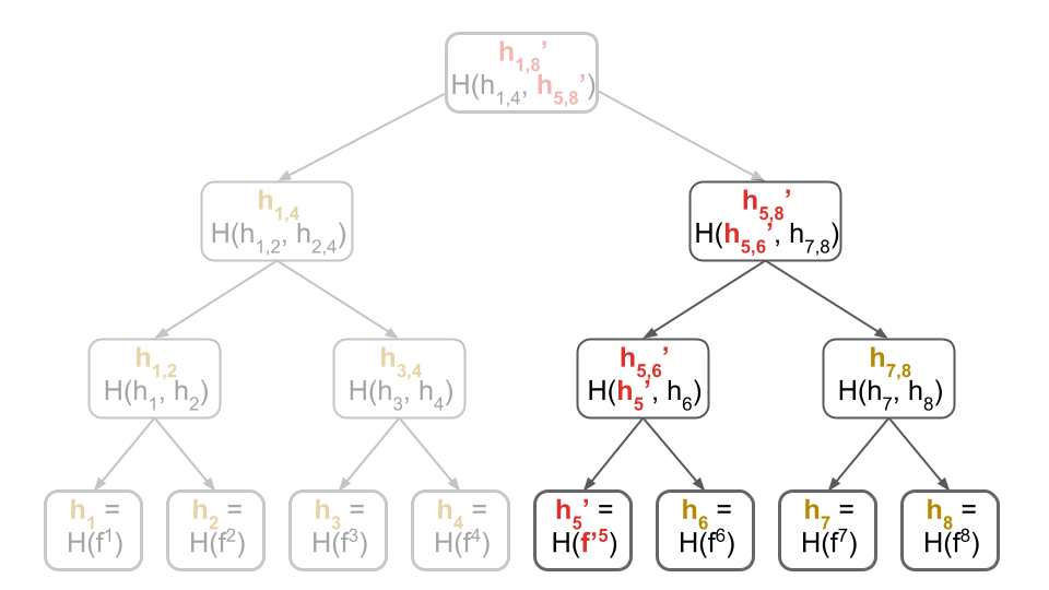
In other words, you have now reduced your initial problem of to a smaller subproblem! Specifically, you must now identify the corrupted block amongst blocks $f^5,\dots,f^8$. And, since you now know that their real Merkle root hash is $h_{5,8}$, you just need to recursively apply the same technique!

Importantly, you should convince yourself that this approach works even if there is more than one corrupted block: you will just have more sub-problems. Furthermore, note that if all blocks are corrupted, then this approach effectively downloads all Merkle hashes in the tree. However, if just one block is corrupted, this approach will only download the hashes along the path to that block (i.e., the ones in red in the figure above) and the Merkle proof for that block (i.e., the sibling nodes of the red nodes).

In general, this approach only downloads (roughly) a Merkle proof per corrupted block, without re-downloading common hashes across different proofs. In contrast, the first solution downloaded one Merkle proof per downloaded block, even if the block was correct!

Generalizing to more than one file

We can generalize the approach above to multiple files. The key idea is to build a Merkle tree over each file’s blocks as already described. If we have $n$ files, we get $n$ Merkle trees with root hashes $r_1, r_2, \dots, r_{n-1}$ and $r_n$, respectively. Next, we build another Merkle tree over these root hashes. Lastly, denote this tree’s root hash by $z_{1,n}$.

For example, here’s what this would look like when $n=8$:

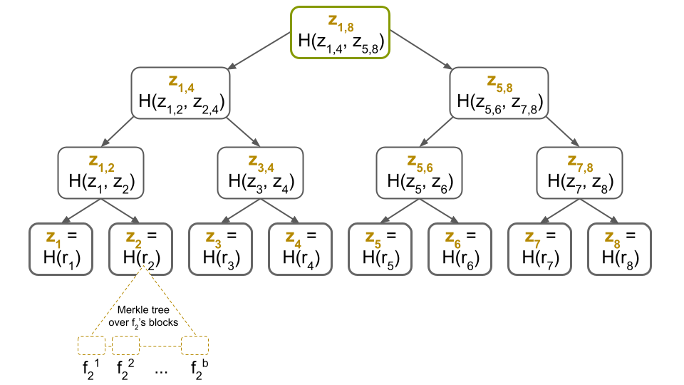
Now, when downloading, say, the 2nd file $f_2$ over an unreliable channel, you first ask for the 2nd leaf of the Merkle tree with root $z_{1,8}$, which is $r_2$, together with a Merkle proof. Once again, because the channel is unreliable, you might have to ask multiple times until the proof verifies. Finally, once you have $r_2$, you can run the protocol described above, since you have the root hash of $f_2$’s Merkle tree!

Want more?

Well, I hope you found all of this fascinating and want to learn more. You could start by going to the bonus section below and reading our formal security proof for Merkle trees.

Then, you could read my three favorite Merkle tree papers, which I think are highly approachable even for beginners.

First, you should read the paper on history trees by Crosby and Wallach⁷. History trees are Merkle trees that “grow” from left to right, in the sense that one is only allowed to append new leafs to the right of the tree.

Despite their simplicity, history trees are incredibly powerful since they support append-only proofs: given an older tree of $t$ leaves and a new tree of $t’=t+\Delta$ leaves, one can prove (using a succinct $O(\log{t’})$-sized proof) that the new tree includes all the leaves from the old tree. This makes history trees very useful for building append-only logs such as Certificate Transparency (CT), which is at the core of securing HTTPS.

“Append-only logs? Don’t you mean blockchains?” you ask. Nope, I do not. These logs have a different mechanism to detect (rather than prevent) forks. However, each fork is always provably extended in append-only fashion using the proofs described above.

Second, you should read the paper on CONIKS by Melara et al⁸. CONIKS is also a transparency log, but geared more towards securing instant messaging apps such as Signal, rather than HTTPS. One interesting thing you’ll learn from this paper is how to lexicographically-order your Merkle trees so you can prove something is not in the tree, as we briefly touched upon in the Bitcoin section. In fact, I believe this paper takes the most sane, straightforward approach to doing so. Specifically, CONIKS builds a Merkle prefix tree, which is much simpler to implement than any binary search tree or treap (at least in my own experience). It also has the advantage of having expected $O(\log{n})$ height if the data being Merkle-ized is not adversarially-produced.

A related paper is would be the Revocation Transparency (RT) manuscript⁹, which CONIKS can be regarded as improving upon in terms of proof size and other dimensions.

Third, you should read the Verifiable Data Structures¹⁰ manuscript by the Certificate Transparency (CT) team, which combines a history tree with a lexicographically-ordered tree (such as CONIKS) into a single system with its own advantages.

At the end of the day, I think what I’m trying to say is “why don’t you go read about transparency logs and come write a blog post on Decentralized Thoughts so I don’t have to do it!” :)

Bonus: A Merkle tree is a collision-resistant hash function

A very simple way to think of a Merkle hash tree with $n$ leaves is as a collision-resistant hash function $\mht$ that takes $n$ inputs¹¹ and ouputs a $2\lambda$-bit hash, a.k.a. the Merkle root hash. More formally, the Merkle hash function is defined as:

And the Merkle root of some input $\vect{x} = (x_1,\dots, x_n)$ is denoted by:

Here, $\lambda$ is a security parameter typically set to 128, which implies Merkle root hashes are 256 bits.

Theorem (Merkle trees are collision-resistant): It is unfeasible to find two sets of leaves $\vect{x} = (x_1, \dots, x_n)$ and $\vect{x}’ = (x_1’, \dots, x_n’)$ such that $\vect{x}\ne \vect{x}’$ but $\mht(\vect{x}) = \mht(\vect{x’})$.

Instead of proving this theorem, we’ll prove an even stronger one below, which implies this one. However, if you want to prove this theorem, all you have to do is show that the existence of these two “inconsistent” sets of leaves implies a collision in the underlying hash function $H$. In fact, in the proof, you will “search” for this collision much like the anti-entropy protocol described above searches for corrupted blocks!

Theorem (Merkle proof consistency): It is unfeasible to output a Merkle root $h$ and two “inconsistent” proofs $\pi_i$ and $\pi_i’$ for two different inputs $x_i$ and $x_i’$ at the $i$th leaf in the tree of size $n$.

Proof: The Merkle proof for $x_i$ is $\pi_i = ((h_1, b_1), \dots, (h_k,b_k))$, where the $h_i$’s are sibling hashes and the $b_i$’s are direction bits. Specifically, if $b_i = 0$, then $h_i$ is a left child of its parent node in the tree and if $b_i=1$, then it’s a right child.

In our previous discussion, we never had to bring up these direction bits because we always visually depicted a specific Merkle proof. However, here, we need to reason about any Merkle proof for any arbitrary leaf. Since such a proof can “take arbitrary left and right turns” as it’s going down the tree, we use these direction bits as “guidance” for the verifier. (A careful reader might notice that the direction bits can actually be derived from the leaf index $i$ being proved and don’t actually need to be sent with the proof: the direction bits are obtained by flipping $i$’s binary representation.)

Roughly speaking, to verify $\pi_i$, the verifier uses $x_i$ together with the sibling hashes and the direction bits to compute the hashes $(z_1, \dots, z_{k+1})$ along the path from $x_i$ to the root. More precisely, the verifier:

1. Sets $z_1 = x_i$.
2. For each $j\in[2,k]$, computes $z_j$ as follows:
   • If $b_{j-1} = 1$, then $z_j = H(z_{j-1}, h_{j-1})$
   • If $b_{j-1} = 0$, then $z_j = H(h_{j-1}, z_{j-1})$

Lastly, the verifier checks if $z_{k+1}$ equals the Merkle root hash $h$. If it does, then the verification succeeds. Otherwise, it fails.

Do not be intimidated by all the math above: we are merely generalizing the Merkle proof verification that we visually depicted in the Dropbox file outsourcing example at the beginning of this post.

Similarly, the proof for $x_i’$ is $\pi_i’ = ((h_1’, b_1), \dots, (h_k’, b_k))$. Note that the $h_i’$ hashes could differ from the $h_i$ hashes, but the direction bits are the same, since both proofs are for the $i$th leaf in the tree.

Since both proofs verify, the verification of the second proof $\pi_i’$ for $x_i’$ will yield hashes $\{z_1’,z_2’,\dots,z_{k+1}’\}$ along the same path from $x_i’$ to the root such that $z_{k+1}’ = h$.

But recall from the verification of the first proof $\pi_i$ that we also have $z_{k+1} = h$. Thus, $z_{k+1} = z_{k+1}’$. This is merely saying that, since both proofs verify, they yield the same root hash $h = z_{k+1} = z’_{k+1}$.

The next step is to reason about how the two different $x_i\ne x_i’$ could have possibly “hashed up” to the same root hash $h$. (Spoiler alert: only by having a collision in the underlying hash function $H$.) I think this is best explained by considering a few extreme cases and then generalizing. (Note that these are not the only two cases; just two particularly enlightening ones.)

Extreme case #1: One way would have been for the proof verification to yield $z_j \ne z_j’$ for all $j\in[k]$ (but not for $j=k+1$ since that’s the level of the Merkle root). In this case, without loss of generality, assume $b_k = 1$. Then, we would have $h = z_{k+1} = H(z_k, h_k)$ and $h = z_{k+1}’ = H(z_k’, h_k’)$. But since $z_k \ne z_k’$, this gives a collision in $H$! (Alternatively, if $b_k = 0$, just switch the inputs to the hash function.)

Extreme case #2: Another way would have been for the proof verification to yield $z_j = z_j’$ for all $j\in[2, k+1]$ (but not for $j=1$ since that’s the level of $x_i$ and $x_i’$ and they are not equal). In this case, without loss of generality, assume $b_1 = 1$. Then, we would have $z_2 = H(x_1, h_1)$ and $z_2’ = H(x_1’, h_1’)$. (Again, if $b_k = 0$, just switch $H$’s inputs.) But since $z_2 = z_2’$ and $x_i\ne x_i’$, this gives a collision in $H$!

The point here is to see that, no matter what the two inconsistent proofs are, one can always work their way back to a collision in $H$, whether that collision is at the top of the tree (extreme case #1), at the bottom of the tree (extreme case #2) or anywhere in between, which we discuss next.

You should now be able to see more easily that, as long as $x_i\ne x_i’$ but the computed root hashes are the same (i.e., $z_{k+1} = z_{k+1}’ = h$), then there must exist some level $j\in [k]$ where there is a collision:

\begin{align*} \exists\ \text{level}\ j\in [k]\ & \text{s.t.}\ \begin{cases} H(z_{j-1}, h_{j-1}) = H(z_{j-1}’, h_{j-1}’),\ \text{if}\ b_{j-1} = 1\\
H(h_{j-1}, z_{j-1}) = H(h_{j-1}’, z_{j-1}’),\ \text{if}\ b_{j-1} = 0 \end{cases} \\
\\
& \text{but with}\ z_{j-1}\ne z_{j-1}’\ \text{or}\ h_{j-1}\ne h_{j-1}’ \end{align*}

(Again, recall that $z_1 = x_i$ and $z_1’=x_i’$.) But such a collision at level $j$ implies a break in the collision-resistance of $H$, which is a contradiction. QED.

The claim about the existence of such a level $j$ might not be easy to understand at first glance. It is best to draw yourself a Merkle proof together with the hashes computed during its verification and run through the following mental exercise:

Start at the root of the tree, at level $k+1$! Since both proofs verify and yield the same root hash, it could be that we either have a collision in $H$ at this level or we don’t. If we do have a collision, we are done. If we do not, then we know that $z_k = z_k’$ and $h_k = h_k’$.

Next, work your way down and continue on the subtree with root hash $z_k = z_k’$. Again, it must be that either there was a collision or that $z_{k-1} = z_{k-1}’$ and $h_{k-1} = h_{k-1}’$. If there was a collision, we are done. Otherwise, we continue recursively.

In the end, we will get to the bottom level which is guaranteed to have $z_1\ne z_1’$ (because $x_i\ne x_i’$) while $z_2 = z_2’$ from the previous level, which yields a collision. This is actually the extreme case #2 that we’ve handled above! No matter what, there will always be a collision!

Acknowledgments

Special thanks to Ittai Abraham for reviewing a draft of this post and sending insightful comments.

References